이 문서에선 convolution기반의 High Pass Filter를 scikit-image 로 사용하는 방법을 다룬다.
https://gist.github.com/dsaint31x/5047a8215fde593b4f1de709fee51b68
scikit-image High Pass Filter.ipynb
scikit-image High Pass Filter.ipynb. GitHub Gist: instantly share code, notes, and snippets.
gist.github.com
opencv버전은 다음을 참고:
https://dsaint31.me/mkdocs_site/DIP/cv2/ch02/dip_edge_detection_high_pass_filter/
BME
High Pass Filter and Edge Detection High Pass Filter image의 spatial frequency domain에서 high frequency 영역을 통과시키는 필터를 가리킴. Fourier transform을 이용하여 구현할 수도 있으나, spatial domain에서 convolution 연산
dsaint31.me
1. High Pass Filter
- image의 spatial frequency domain에서 high frequency 영역을 통과시키는 필터를 가리킴.
- Fourier transform을 이용하여 구현할 수도 있으나, spatial domain에서 convolution 연산을 통해서도 구현 가능함.
https://dsaint31.me/mkdocs_site/DIP/cv2/etc/dip_convolution/
BME
convolution filter kernel Convolution 이 문서에서의 convolution은 digital image processing등에서의 convolution을 다루고 있음. signal processing의 discrete convolution에 대한 건 다음 문서를 참고할 것: Discrete Convolution, Cir
dsaint31.me
High Pass Filter의 특징.
- Edge Detection, Sharpening이 이루어짐.
- HPF는 영상에서 낮은 주파수 성분을 제거하여, 물체의 윤곽선이나 세부정보를 강조하는 edge를 검출할 수 있음
- 영상의 경계선이 더욱 선명해지는 sharpening 영상을 얻을 수 있지만, 오히려 잡음을 증가시켜 화질이 약화될 수 있음
- 단, Noise도 같이 강조됨
참고: Differentiation(미분) and Difference(차분)
digital image에선 gradient 연산을 미분(differentiation)의 근사인 차분(difference)을 통해 구현함.
https://dsaint31.tistory.com/540
[Math] Differentiation (or Differential, 미분)과 Difference (차분)
Derivative 란?"Differential을 구한다(Differentiation, 미분하다)" 는 derivative(도함수)를 구하는 것을 가르킴. Derivative(도함수)는average rate of change (평균변화율)의 limit인instantaneous rate of change (=derivative value,
dsaint31.tistory.com
difference(차분)도 convolution을 통해 쉽게 구현 가능함.
아쉽게도 scikit-image에는 다른 라이브러리의 convolve나 filter2d 와 같은 커널을 지정하여 convolution을 하는 함수가 없음.
때문에 scipy.ndimage.convolve를 대신 이용하는 경우가 많음 (ndarray지원 및 경계처리 옵션이 다양함).
from scipy.ndimage import convolve
from skimage import io, color, img_as_float
import numpy as np
import matplotlib.pyplot as plt


# 1. 이미지 불러오기 (예: Sudoku 이미지)
url = "https://raw.githubusercontent.com/dsaint31x/OpenCV_Python_Tutorial/master/images/sudoku.jpg"
img = io.imread(url)

img = color.rgb2gray(img_as_float(img))   # [0,1] float 범위로 변환

# 2. Forward Difference 커널 정의
gx_kernel = np.array([[-1, 1]], dtype=float)   # x 방향 (가로 미분)
gy_kernel = np.array([[-1], [1]], dtype=float) # y 방향 (세로 미분)

# 3. 컨볼루션 수행 (scipy.ndimage.convolve 또는 skimage.filters.apply_hysteresis_threshold 등 사용 가능)
x_edge = convolve(img, gx_kernel, mode='reflect')
y_edge = convolve(img, gy_kernel, mode='reflect')
# 절댓값 처리
x_edge_abs = np.abs(x_edge)
y_edge_abs = np.abs(y_edge)

# 4. 시각화
# results = np.hstack((img,x_edge_abs,y_edge_abs))
# plt.figure(figsize=(10,30))
# plt.imshow(results, cmap='gray')
# plt.axis("off")
# plt.show()

# subplot으로 나란히 표시
fig, axes = plt.subplots(1, 3, figsize=(12, 4))

axes[0].imshow(img, cmap='gray')
axes[0].set_title('Original')
axes[0].axis('off')

axes[1].imshow(x_edge_abs, cmap='gray')
axes[1].set_title('|X Edge| (Forward diff)')
axes[1].axis('off')

axes[2].imshow(y_edge_abs, cmap='gray')
axes[2].set_title('|Y Edge| (Forward diff)')
axes[2].axis('off')

plt.tight_layout()
plt.show()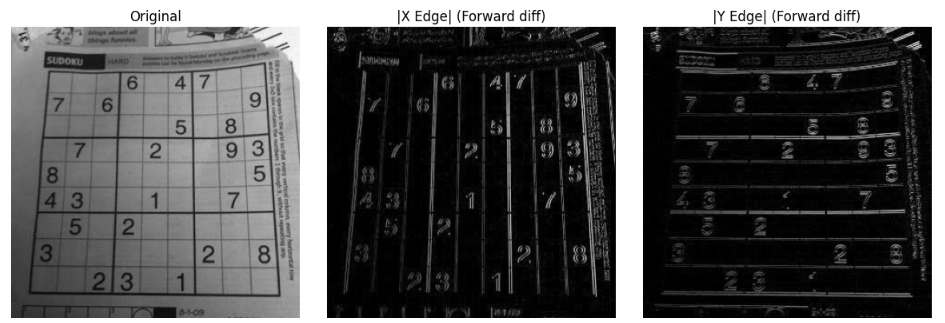
2. Gradient 기반 filters
1차 미분 기반을 가리킴. 일반적으로 x축, y축의 gradient를 구하고 이들을 이용하여 magnitude를 구하는 게 일반적임.
Gradient는 pixel intensity가 가장 가파르게 증가하는 direction 과 그 증가하는 변화율의 크기를 magnitude로 가지는 vector임.
Gradient의 magnitude는 x,y축의 gradient를 구하고 이들을 $\sqrt{g_x^2 +g_y^2}$을 통해 magnitude를 구함.
direction은 $\theta = \text{atan}\left( \frac{g_y}{gx}\right)$로 구함.
https://dsaint31.tistory.com/543
[Math] Gradient (구배, 기울기, 경사, 경도) Vector
Gradient (구배, 기울기, 경사, 경도), $\nabla f(\textbf{x})$Multi-Variate Function (=Scalar Field, Multi-Variable Function) $f(\textbf{x})$에서 input $\textbf{x}$의 미세한 변화에 대해 (scalar) output이 1) 가장 가파르게 증가하
dsaint31.tistory.com
2-1. Lawrence Roberts Filter (Cross Filter)
- 1963년 로렌스 로버츠 제안.
- diagonal edge를 매우 잘 검출.
- noise에 약하고, 검출된 edge강도가 낮은 편.
Roberts Cross Filter는 아주 작은 2×2 커널을 사용해서 대각선 방향의 1차 미분(Gradient) 을 근사.
$$
G_x =
\begin{bmatrix}
+1 & 0 \\
0 & -1
\end{bmatrix},
\quad
G_y =
\begin{bmatrix}
0 & +1 \\
-1 & 0
\end{bmatrix}
$$
이 두 필터를 각각 컨볼루션한 뒤, 에지 강도(gradient magnitude)는 다음과 같이 계산.
$$G = \sqrt{G_x^2 + G_y^2}$$
import matplotlib.pyplot as plt
from skimage import data, color, img_as_float
from skimage.filters import roberts

# 예제 이미지
img = color.rgb2gray(img_as_float(data.astronaut()))

# Roberts 필터 적용
edge_roberts = roberts(img)

# 시각화
fig, ax = plt.subplots(1, 2, figsize=(10, 4))
ax[0].imshow(img, cmap='gray')
ax[0].set_title("Original")
ax[0].axis('off')

ax[1].imshow(edge_roberts, cmap='gray')
ax[1].set_title("Roberts (Lawrence Roberts Filter)")
ax[1].axis('off')
plt.show()

2-2. Prewitt Filter
- 1970년 경 주디스 프리윗(Judith M. S. Prewitt)이 제안
- Centered difference의 digital version이라고 볼 수 있음.
- It shows weak performance for diagonal edge detection.
Sobel mask의 경우와 유사한 성능에 좀더 빠른 응답시간을 보임.
단, Soble에 비해 밝기 변화에 대하여 비중이 약간 적게 준 관계로 edge가 덜 부각 됨.
Roberts가 2×2 대각선 방향을 본다면,
Prewitt은 3×3 커널로 수평/수직 방향 Gradient를 계산.
Prewitt은 다음 두 커널을 사용.
$$G_x =
\begin{bmatrix}
-1 & 0 & +1 \\
-1 & 0 & +1 \\
-1 & 0 & +1
\end{bmatrix},
\quad
G_y =
\begin{bmatrix}
-1 & -1 & -1 \\
0 & 0 & 0 \\
+1 & +1 & +1
\end{bmatrix}
$$
- x방향은 수직 방향 밝기 변화(세로 경계),
- y방향은 수평 방향 밝기 변화(가로 경계)를 검출.
Gradient magnitude:
$$
G = \sqrt{G_x^2 + G_y^2}
$$
import matplotlib.pyplot as plt
from skimage import data, color, img_as_float
from skimage.filters import prewitt

# 예제 이미지 (0~1 float)
img = color.rgb2gray(img_as_float(data.astronaut()))

# Prewitt 필터 적용
edge_prewitt = prewitt(img)

# 시각화
fig, ax = plt.subplots(1, 2, figsize=(10, 4))
ax[0].imshow(img, cmap='gray')
ax[0].set_title("Original")
ax[0].axis('off')

ax[1].imshow(edge_prewitt, cmap='gray')
ax[1].set_title("Prewitt (Judith Prewitt Filter)")
ax[1].axis('off')
plt.show()prewitt()함수는 기본 패딩이 mode="reflect"를 사용함.

convolve를 이용한 방식은 다음과 같음:
import numpy as np
from scipy.ndimage import convolve

# Prewitt 커널 (x, y 방향)
Gx = np.array([[-1, 0, 1],
               [-1, 0, 1],
               [-1, 0, 1]], dtype=float)
Gy = np.array([[-1, -1, -1],
               [ 0,  0,  0],
               [ 1,  1,  1]], dtype=float)

# Convolution
gx = convolve(img, Gx, mode='reflect')
gy = convolve(img, Gy, mode='reflect')

# Gradient magnitude
edge = np.hypot(gx, gy)

# 시각화
fig, ax = plt.subplots(1, 3, figsize=(12, 4))
ax[0].imshow(gx, cmap='gray'); ax[0].set_title("Gx (vertical edges)"); ax[0].axis('off')
ax[1].imshow(gy, cmap='gray'); ax[1].set_title("Gy (horizontal edges)"); ax[1].axis('off')
ax[2].imshow(edge, cmap='gray'); ax[2].set_title("Gradient magnitude"); ax[2].axis('off')
plt.tight_layout(); plt.show()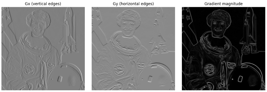
2-3. Sobel Filter
- 1968년 Irwin Sobel과 Gary Feldman이 제안한 필터로,
- Prewitt과 마찬가지로 gradient기반 HPF.
Prewitt보다
부드럽고, 노이즈에 강하며,
방향 응답이 더 안정적
차이점:
- Sobel은 커널에 가우시안 스무딩 효과를 내는 가중치를 포함하여
- 노이즈에 덜 민감하고 연속적인 에지를 잘 검출.
커널 정의 (3×3 기준)
$$
G_x =
\begin{bmatrix}
-1 & 0 & +1 \\
-2 & 0 & +2 \\
-1 & 0 & +1
\end{bmatrix},
\quad
G_y =
\begin{bmatrix}
-1 & -2 & -1 \\
0 & 0 & 0 \\
+1 & +2 & +1
\end{bmatrix}$$
- Prewitt과 비슷하지만 가중치(2)가 중앙 행/열에 들어가 있어
- 수평·수직 방향 변화에 더 부드럽게 반응.
Gradient magnitude는 다음과 같음:
$$
G = \sqrt{G_x^2 + G_y^2}
$$
import matplotlib.pyplot as plt
from skimage import data, color, img_as_float
from skimage.filters import sobel

# 예제 이미지
img = color.rgb2gray(img_as_float(data.astronaut()))

# Sobel 필터 적용
edge_sobel = sobel(img)

# 시각화
fig, ax = plt.subplots(1, 2, figsize=(10, 4))
ax[0].imshow(img, cmap='gray')
ax[0].set_title("Original")
ax[0].axis('off')

ax[1].imshow(edge_sobel, cmap='gray')
ax[1].set_title("Sobel Filter")
ax[1].axis('off')
plt.show()sobel()함수는 기본 패딩이 mode="reflect"를 사용함.

참고: Sobel vs Prewitt vs Roberts 비교
| 항목 | Roberts | Prewitt | Sobel |
| 커널 크기 | 2×2 | 3×3 | 3×3 |
| 방향 | 대각선 | 수평/수직 | 수평/수직 |
| 스무딩 효과 | 없음 | 없음 | 있음 (가중치 2) |
| 노이즈 민감도 | 높음 | 중간 | 낮음 |
| 계산 복잡도 | 매우 낮음 | 낮음 | 약간 높음 |
| scikit-image 함수 | filters.roberts() |
filters.prewitt() |
filters.sobel() |
2-4. Scharr Filter
- 2000년대 초, H. Scharr(독일 하이델베르크 대학, 2000)이 제안한 gradient기반 HPF
- Sobel과 유사
- 단, 고정된 3×3 Kernel을 사용하면서
- 방향성(회전 불변성, rotational symmetry)을 더욱 개선하기 위해 커널의 가중치를 최적화함.
Sobel은 3×3 커널에서 회전 대칭성이 완전하지 않아
45°, 135° 방향의 에지 검출이 조금 왜곡될 수 있는 단점을 가지나
Scharr은 이 문제를 최소화시킴.
하지만 Sobel은 다양한 kernel size가 가능하나,
Scharr는 3x3 고정임 (이 사이즈에 최적화 됨).
Scharr 커널 (3×3 고정)
$$
G_x =
\begin{bmatrix}
-3 & 0 & +3 \\
-10 & 0 & +10 \\
-3 & 0 & +3
\end{bmatrix},
\quad
G_y =
\begin{bmatrix}
-3 & -10 & -3 \\
0 & 0 & 0 \\
+3 & +10 & +3
\end{bmatrix}
$$
- 즉, Sobel의 [-1, -2, -1] 대신 [-3, -10, -3]으로 가중치를 강화
- 중심부 스무딩 + 방향성 정확도를 모두 향상시킴.
import matplotlib.pyplot as plt
from skimage import data, color, img_as_float
from skimage.filters import scharr

# 예제 이미지
img = color.rgb2gray(img_as_float(data.astronaut()))

# Scharr 필터 적용
edge_scharr = scharr(img)

# 시각화
fig, ax = plt.subplots(1, 2, figsize=(10, 4))
ax[0].imshow(img, cmap='gray')
ax[0].set_title("Original")
ax[0].axis('off')

ax[1].imshow(edge_scharr, cmap='gray')
ax[1].set_title("Scharr Filter")
ax[1].axis('off')
plt.show()scharr()함수는 기본 패딩이 mode="reflect"를 사용함.

수동 커널 구현
import numpy as np
from scipy.ndimage import convolve

# Scharr 커널
Gx = np.array([[-3, 0, 3],
               [-10, 0, 10],
               [-3, 0, 3]], dtype=float)
Gy = np.array([[-3, -10, -3],
               [ 0,   0,  0],
               [ 3,  10,  3]], dtype=float)

# Convolution
gx = convolve(img, Gx, mode='reflect')
gy = convolve(img, Gy, mode='reflect')

# Gradient magnitude
edge = np.hypot(gx, gy)

# 시각화
fig, ax = plt.subplots(1, 3, figsize=(12, 4))
ax[0].imshow(gx, cmap='gray'); ax[0].set_title("Gx (vertical edges)"); ax[0].axis('off')
ax[1].imshow(gy, cmap='gray'); ax[1].set_title("Gy (horizontal edges)"); ax[1].axis('off')
ax[2].imshow(edge, cmap='gray'); ax[2].set_title("Magnitude (Scharr)"); ax[2].axis('off')
plt.tight_layout(); plt.show()
참고: Sobel vs. Scharr Filter
| 항목 | Sobel | Scharr |
| 커널 크기 | 3×3, 5×5 등 확장 가능 | 3×3 고정 |
| 가중치 중심 행/열 | ±1, ±2 | ±3, ±10 |
| 회전 불변성 (Rotational Symmetry) |
부분적 — 45°, 135° 방향에서 약간의 왜곡 존재 | 매우 우수 — 회전 대칭성 최적화 |
| 노이즈 억제 (Noise Suppression) |
우수 (가중치에 의한 스무딩 효과) | 우수 (가중치 최적화) |
| 방향 정확도 (Directional Accuracy) |
보통 | 높음 |
| scikit-image 함수 | skimage.filters.sobel() |
skimage.filters.scharr() |
| 특징 요약 | Sobel은 다양한 커널 크기로 확장 가능하며 일반적인 엣지 검출에 널리 사용됨 | Scharr은 3×3 범위에서 방향성(회전 불변성)을 최적화한 정밀 gradient 기반 HPF |
- Sobel은 확장성과 단순성이 장점이며,
- Scharr은 동일한 3×3 크기에서 회전 대칭성과 방향 정확도를 극대화한 고정 커널 필터.
Scharr은 특히 정밀한 방향 정보가 필요한 경우 (예: 에지 방향 기반 특징, Optical Flow, Gradient Orientation Histogram 등) Sobel보다 더 적합함.
2-5. Roberts ~ Scharr 정리 비교표
| Filter | 커널 크기 | 방향성 | 노이즈 민감도 | 회전 정확도 | scikit-image 함수 |
| Roberts | 2×2 | 대각 | 매우 높음 | 낮음 | filters.roberts() |
| Prewitt | 3×3 | 수평 / 수직 | 중간 | 중간 | filters.prewitt() |
| Sobel | 3×3 (확대가능) | 수평 / 수직 | 낮음 | 중간 | filters.sobel() |
| Scharr | 3×3 (고정) | 수평 / 수직 | 낮음 | 높음 | filters.scharr() |
3. Laplacian Filter
2차 미분 필터 (The 2nd Order Derivative Filter)
- 1차 미분 필터(예: Sobel Filter)과 비교할 경우,
영상 내의 blob이나 섬세한(fine) 구조를 더 잘 검출(또는 강조)함. - 단점: 노이즈까지 함께 강조됨 : 매우 노이즈에 취약함.
- 따라서 사전에 Gaussian Blurring을 적용하는 것이 일반적임.
- 2차 미분 필터는 주로 image enhancement(영상 강조)에 사용되며,
1차 미분 필터는 feature extraction(특징 추출)에 더 자주 사용됨.
Laplacian of Gaussian (LoG)
Laplacian은 노이즈에 매우 민감하기 때문에 단독으로 사용하기보다는
Gaussian Filter로 블러링하여 노이즈를 제거한 후
Laplacian Filter를 적용하는 방식(LoG)이 일반적으로 사용됨.
LoG는 Laplacian이 noise에 취약한 점을 극복하기 위해 일종의 band-pass filter임
(Difference of Gaussians가 LoG를 대체하는 경우도 많음)
import numpy as np
import matplotlib.pyplot as plt
from skimage import io, color, img_as_float
from skimage.filters import laplace, gaussian

# 1) 이미지 로드 (0~1 float)
url = "https://raw.githubusercontent.com/dsaint31x/OpenCV_Python_Tutorial/master/images/sudoku.jpg"
img_rgb = io.imread(url)
img = color.rgb2gray(img_as_float(img_rgb))

# 2) Laplacian (ksize는 홀수 >=3)
edge_lap = laplace(img, ksize=3)
edge_lap_abs = np.abs(edge_lap)

# 3) LoG: Gaussian → Laplacian
blur = gaussian(img, sigma=1.0, preserve_range=True)
edge_log = np.abs(laplace(blur, ksize=3))

# 4) 시각화
fig, axes = plt.subplots(1, 3, figsize=(12, 4))
axes[0].imshow(img, cmap='gray');          axes[0].set_title("Original");            axes[0].axis('off')
axes[1].imshow(edge_lap_abs, cmap='gray'); axes[1].set_title("Laplacian (|edge|)");  axes[1].axis('off')
axes[2].imshow(edge_log, cmap='gray');     axes[2].set_title("LoG (Gaussian→Lap)");  axes[2].axis('off')
plt.tight_layout(); plt.show()
laplace는 내부적으로 scipy.ndimage.convolve()를 사용하기 때문에 패딩이 "reflect"로 이루어진다 (변경을 인자로 할 수 없음)

다음과 같이 직접 scipy.ndimage.convolve()로 라플라시안 커널을 직접 적용한 버전을 사용하면 padding 변경이 가능함.
from scipy.ndimage import convolve

kernel_lap = np.array([[0,  1, 0],
                       [1, -4, 1],
                       [0,  1, 0]], dtype=float)   # 3×3 라플라시안(4-이웃)

edge_lap_manual = convolve(img, kernel_lap, mode='reflect')
edge_lap_manual_abs = np.abs(edge_lap_manual)

fig, axes = plt.subplots(1, 2, figsize=(8, 4))
axes[0].imshow(img, cmap='gray')
axes[0].set_title("Original")
axes[0].axis('off')
axes[1].imshow(edge_lap_manual_abs, cmap='gray')
axes[1].set_title("Laplacian (|edge|)")
axes[1].axis('off')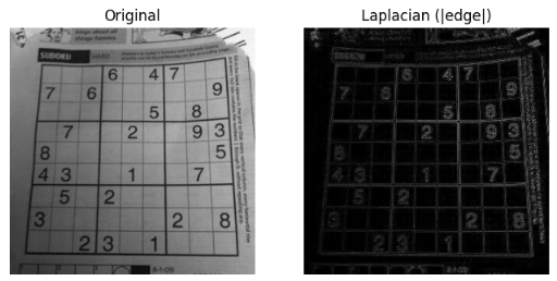
같이 보면 좋은 자료들
2025.10.21 - [Python] - scikit-image: Low Pass Filter
scikit-image: Low Pass Filter
Low Pass Filter (LPF)1. Filter란?Filter란 입력 영상으로부터원하지 않는 성분을 걸러내고,필요한 성분만을 통과시켜 추출하는 방법 또는 연산(컴포넌트)을 의미함.2. Low Pass Filter란?Low Pass Filter는 영상의
ds31x.tistory.com
https://dsaint31.me/mkdocs_site/DIP/cv2/ch02/dip_low_pass_filter/
BME
Low Pass Filter filter란 입력이미지에서 원하지 않는 값들은 걸러내고 원하는 값들을 추출하여 결과로 얻는 방법 또는 컴포넌트를 지칭. 대표적인 예로 edge 의 위치와 방향을 검출하여 Image Analysis 및
dsaint31.me
2025.07.01 - [Python] - Pillow 사용법 - Basic 04 - ImageFilter
Pillow 사용법 - Basic 04 - ImageFilter
PIL.ImageFilter는 이미지에blur, sharpening, edge detection, emboss 등다양한 시각적 효과를 적용할 수 있는 사전 정의된 필터들을 제공하는 모듈.이는 convoluton 기반으로 동작하는 다양한 필터를 사전 정의하
ds31x.tistory.com
https://dsaint31.me/mkdocs_site/DIP/ch10_LoG/
BME
Laplacian of Gaussian (LoG) LoG는 Marr과 Hildreth에 의해 1980년에 제안된 기법. Gaussian blurring을 사용하여 noise를 제거(or 완화)시킨 후 Laplacian을 가하여 edge를 추출. Laplacian이 edge를 잘 찾아내는 장점을 가지
dsaint31.me
'Python' 카테고리의 다른 글
| Recursive Function and Recurrence Relation (1) | 2025.12.05 |
|---|---|
| scikit-image: Low Pass Filter (0) | 2025.10.21 |
| scikit-image: Image Load, Save, Display (0) | 2025.10.20 |
| skimage 에서 image 정보, color space 변경 및 histogram 생성. (0) | 2025.10.20 |
| zip import 튜토리얼-__init__.py 와 __main__.py (0) | 2025.10.17 |


